Introduction

SQL is a declarative language, which means that when you request a query, you specify the data you want, but not how to get it. The database management system (DBMS) is responsible for determining the most efficient way to retrieve the requested data. This separation of concerns allows users to focus on what data they need, while the DBMS can optimize the underlying operations for efficiency and performance.

There are two main approaches to optimizing a query: heuristics and cost-based search.

Heuristics optimization involves using a set of pre-defined rules or patterns to determine the most efficient way to execute a query. These rules are based on common patterns and practices that are effective in many cases, but they may not always produce the most optimal plan.

Cost-based optimization involves using statistical information about the data and the query itself to determine the most efficient execution plan. The DBMS estimates the costs of different potential execution plans and chooses the one with the lowest cost. This approach can be more accurate than heuristics optimization, but it can also be more time-consuming.

Heuristics & Rules

During query optimization, the database management system (DBMS) will attempt to rewrite the original query provided by the user in a more efficient form. This may include removing unnecessary conditions and using the system catalog (a repository of information about the database's structure and contents) to identify more efficient ways to retrieve the requested data.

The DBMS may also use techniques from relational algebra, a set of mathematical operations used to manipulate data stored in a relational database, to identify equivalent expressions that can be used to achieve the same result. This process allows the DBMS to identify multiple ways to execute the same query and choose the most efficient option.

Predicate Pushdown

Example query

SELECT s.name, e.cid
FROM student AS s, enrolled AS e
WHERE s.sid = e.sid
AND e.grade = 'A'

Expression: π(name,id)(σgrade='A'(student⋈enrolled))

Equivalent to: π(name, id)(student⋈(σgrade='A'(enrolled)))

If two equivalent expressions can be used to achieve the same result in a query, why might the database management system (DBMS) choose one over the other?

In our case, the second expression filters the record from table e before performing a join, it's more efficient because it reduces the amount of work the join operation needs to do. The DBMS can more efficiently retrieve the desired data by eliminating unnecessary records.

Re-order predicates

It may also be that a specific predicate is more selective than another one, so it's more convenient to push it down before the others.

Simplify complex predicates

As we know, DBMS executes the predicate to every tuple it receives from the scan operator, if the predicate can be optimized to have less CPU and memory usage, then it's a huge win!

SELECT first_name, last_name, film_id
FROM actor a
JOIN film_actor fa ON a.actor_id = fa.actor_id
WHERE a.actor_id = 1;

can be re-written into:

SELECT first_name, last_name, film_id
FROM actor a
JOIN film_actor fa ON fa.actor_id = 1
WHERE a.actor_id = 1;

Projection Pushdown

When we have a projection, it will be better if we did it before passing data from one operator to another as it reduces the memory used by the query. Thus, reducing I/O too.

Impossible Predicates

Sometimes applications issue impossible predicates, that are coming from a user playing around with values from the dashboard somewhere. It would be cool if DBMS detected those and didn't spend time executing them.

SELECT * FROM A WHERE 1 = 0;
SELECT * FROM A WHERE 1 = 1;

Merging Predicates

Sometimes predicates are overlapped, and merging reduces CPU utilization

SELECT * FROM A
WHERE val BETWEEN 1 AND 100
OR val BETWEEN 50 AND 150;

DBMS decides to merge them into:

SELECT * FROM A
WHERE val BETWEEN 1 AND 150;

Cost-based Search

In this model, DBMS uses actual data from the tables to determine which plan is better. Unlike the previous way, in which we use static rules. This one evaluates multiple query plans and chooses only the one that has the lowest cost.

The main idea here is to store some statistics about each table, and its attributes (indexes also). And use those statistics to determine the best plan.

Statistics

For each relation R, DBMS stores: Nr which is the number of the records in R, V(A, R): the number of the distinct values for each attribute A. Using those two values, we can do some good calculations.

Selection cardinality is the average number of records with a value for a given attribute, SC(A, R) = Nr/V(A, R)

Selectivity of a predicate is the fraction of tuples that qualifies for this predicate

Assumptions

There's a trade-off between having accurate cost analysis and storage, if we want to have a high-accuracy model, then we need bigger storage. However, those statistics should be minimal because we are going to use them in every query, so it's crucial to keep them in memory, not on the disk. That's why we assume data is uniform, and collect some statistics assuming it accurately represents the actual data (which is not the case).

We are assuming that there are no data dependencies, which means that no attribute value affects another attribute. In the real world, a specific city would have a specific postal code, so there's a dependency here. However, we are assuming it's not happening in our DB. Some enterprise databases might allow you to define those dependencies, but it's not common.

Sampling

Some databases collect samples from real tables to estimate selectivity. Which requires updating the sample when the tables are changed. Another trade-off, we decide to update the samples when only significant changes happen to the table because we don't need to waste too much effort on keeping samples updated. However, we sacrifice keeping samples accurate, but it's acceptable.

Query Optimization

Since we know how to estimate the cost of the plan, it's time to enumerate different plans for the query and estimate their costs, then decide which one should be executed.

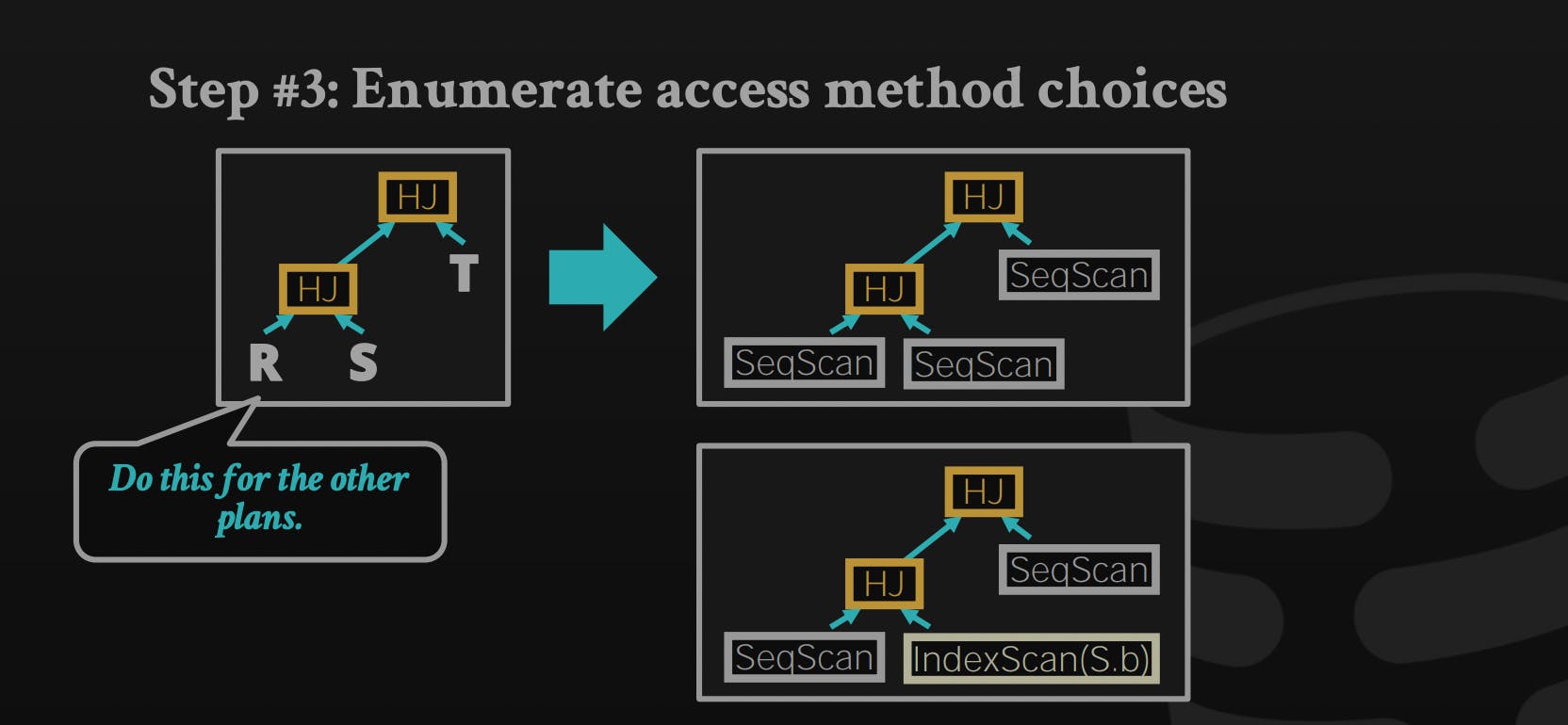
• Single-relation query: pick the best access method, which is one of the sequential scans, binary search (clustered indexes), or index scan.

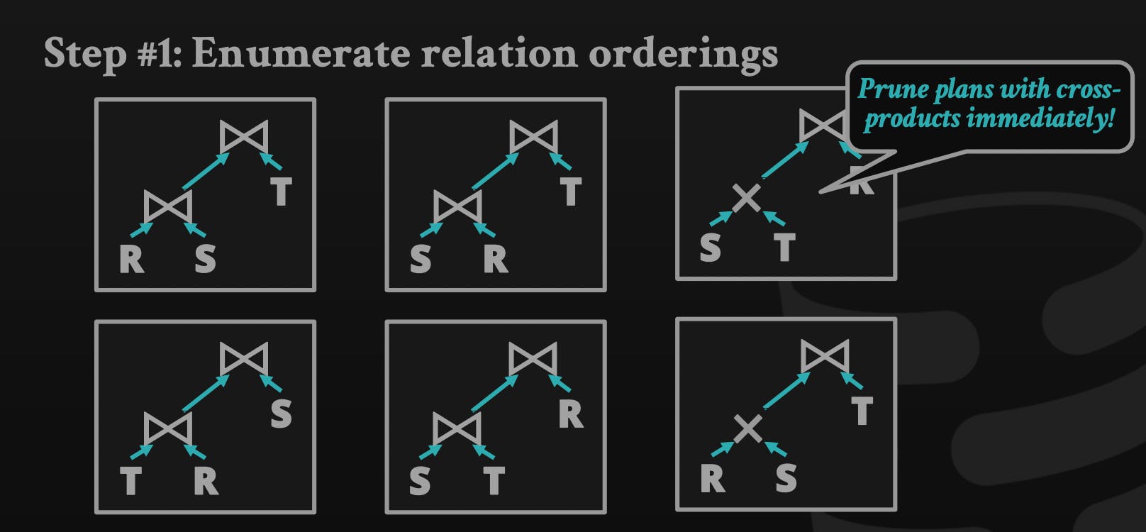
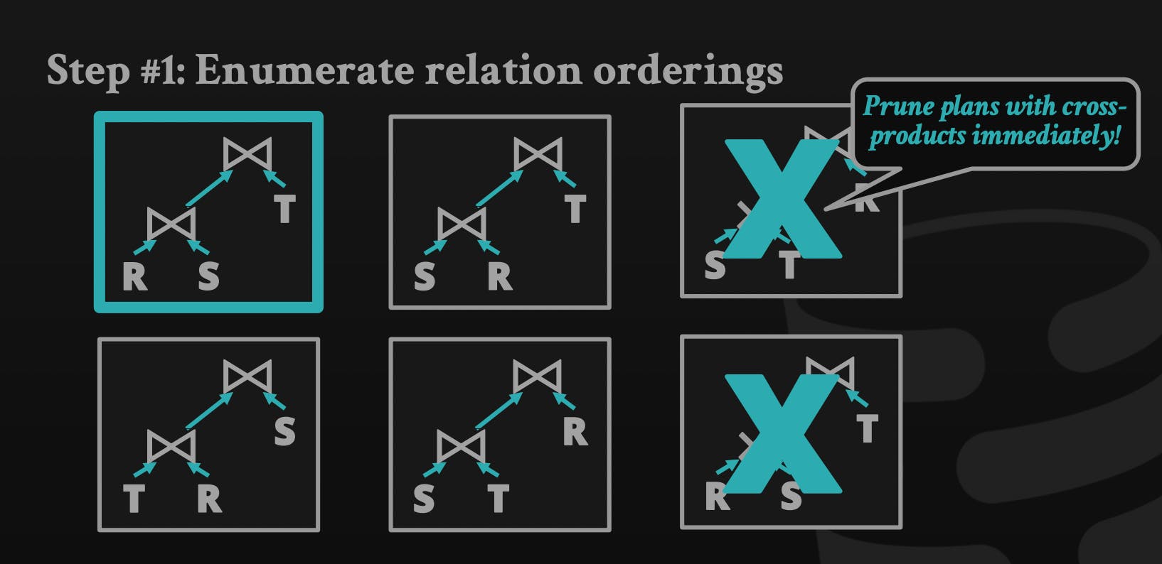
• Multi-relation query: as joins increase, alternative plans grow exponentially.

In general, the algorithm to generate different plans:

1. Enumerate relation ordering

   

   

2. Enumerate joins algorithm choices

   

1. Enumerate access method choices

   

Nested Sub-Queries

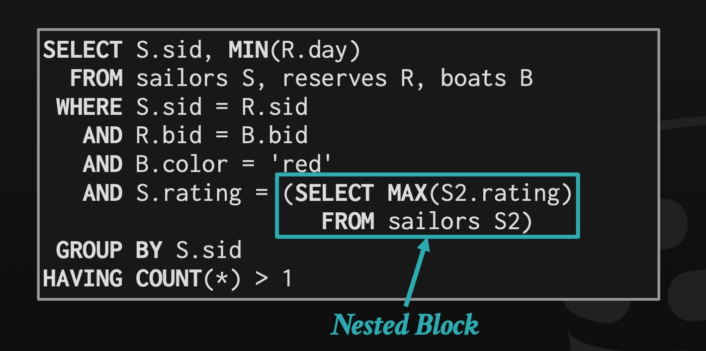
There are two different approaches to optimizing nested sub-queries.

1. Rewrite the query to de-correlate them.

   

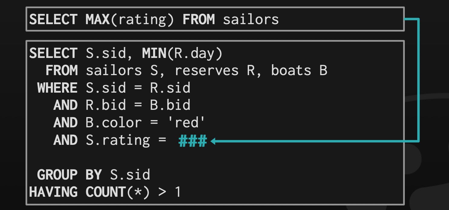
2. Decompose nested queries and store results in a temporary table.

   

   

   References

   • CMU15-445/645 Database Systems lecture notes. Retrieved from: 15445.courses.cs.cmu.edu/fall2019

     Note: ChatGPT was used to help me refine and make this post more concise, and readable, and provided some examples. So huge thanks to OpenAI!